
Does Buying the Dip Work? Short-Term Reversal by Volatility Regime in Python
August 11, 2026
What’s the question?
Short-term reversal is the claim that a fall today is partly repaid tomorrow. It sits underneath most oversold indicators, the two-day RSI and the lower Bollinger band among them, and it is usually stated without conditions: buy weakness, always.
There is a reason to doubt the unconditional version. A one-day bounce forecasts nothing fundamental, since nothing about a company changes between two consecutive closes. The plausible source is payment for liquidity: when a wave of selling arrives, someone has to take the other side, and that someone charges a price concession for absorbing inventory they did not want, which unwinds over the following day. That story predicts a bounce that scales with how expensive risk-taking is at the time: large when volatility is elevated, absent when markets are quiet.
The question is therefore not whether dip buying works, but when.
The approach
The test covers eight exchange-traded funds: SPY (US large cap), IWM (US small cap), EFA (developed markets outside the US), EEM (emerging markets), XLK (technology), XLP (consumer staples), TLT (long Treasuries), and GLD (gold). Bonds and gold are in the sample deliberately: a payment for absorbing equity risk should be weak in assets that do not carry it.
- Pull daily total returns for each fund from January 2004 to August 2026, so that dividend dates do not register as artificial falls.
- Compute the standard deviation of the last 20 daily returns on every date.
- Rank that volatility against its own trailing two-year history and split the days into thirds: calm, normal, stressed. The rank uses only data available on the day, so no fund is labelled stressed because of a crisis that had not yet happened. The burn-in leaves a window starting in January 2006.
- Split every day by the sign of that day’s return and measure the next close-to-close return.
- Define the reversal spread as the mean next-day return after a down day minus the mean after an up day, with standard errors clustered on date, since the eight funds fall together.
Code
import numpy as np
import pandas as pd
import xfinlink as xfl

xfl.set_api_key("YOUR_API_KEY")  # free at https://xfinlink.com/signup

tickers = ["SPY", "IWM", "EFA", "EEM", "XLK", "XLP", "TLT", "GLD"]
px = pd.concat([xfl.prices(t, start="2004-01-01", end="2026-08-07",
                           fields=["return_daily"]) for t in tickers],
               ignore_index=True).sort_values(["ticker", "date"])

def build(g):
    g = g.copy()
    r = g["return_daily"]
    g["vol"] = r.rolling(20).std()
    g["pct"] = g["vol"].rolling(504).apply(lambda w: (w[:-1] < w[-1]).mean(), raw=True)
    g["fwd"] = r.shift(-1)
    return g

panel = pd.concat([build(g) for _, g in px.groupby("ticker")], ignore_index=True)
panel = panel.dropna(subset=["pct", "fwd"])
panel["regime"] = pd.cut(panel["pct"], [-0.001, 1/3, 2/3, 1.001],
                         labels=["calm", "normal", "stressed"])
panel["down"] = (panel["return_daily"] < 0).astype(float)

def spread(frame):
    """Mean next-day return after a down day minus after an up day,
    with standard errors clustered on date."""
    X = np.column_stack([np.ones(len(frame)), frame["down"].values])
    y = frame["fwd"].values
    A = np.linalg.inv(X.T @ X)
    b = A @ X.T @ y
    u = y - X @ b
    meat = np.zeros((2, 2))
    for idx in frame.groupby("date").indices.values():
        s = X[idx].T @ u[idx]
        meat += np.outer(s, s)
    return b[1], b[1] / np.sqrt((A @ meat @ A)[1, 1])

for regime in ["calm", "normal", "stressed"]:
    sp, t = spread(panel[panel["regime"] == regime])
    print(f"{regime}: spread {sp * 1e4:.2f} bp, t {t:.2f}")
Full script with formatting and visualisation: does-buying-the-dip-work-volatility-regime-python.py
Output
SPY IWM EFA EEM XLK XLP TLT GLD: daily total returns 2004-01-02 to 2026-08-07, 45,250 bars, 41,065 usable observations
regime = trailing two-year percentile of the 20-day return standard deviation

next-day return, pooled across the eight funds
regime        days   after a down day   after an up day    spread      t
calm        14,860            2.91 bp           1.87 bp   1.05 bp   0.50
normal      11,924            9.20 bp           1.70 bp   7.51 bp   2.90
stressed    14,281           16.42 bp          -4.67 bp  21.10 bp   3.88

reversal spread by fund (basis points, t in brackets)
fund                 calm          stressed
SPY         -2.19 (-0.64)     21.33 ( 2.50)
IWM          4.22 ( 0.84)     16.09 ( 1.57)
EFA          3.51 ( 0.90)     23.86 ( 2.68)
EEM         -7.19 (-1.39)     50.41 ( 4.33)
XLK         -0.48 (-0.10)     27.28 ( 3.00)
XLP          6.06 ( 2.06)     17.19 ( 3.09)
TLT          5.52 ( 1.70)      1.64 ( 0.29)
GLD         -0.15 (-0.04)      8.50 ( 1.16)

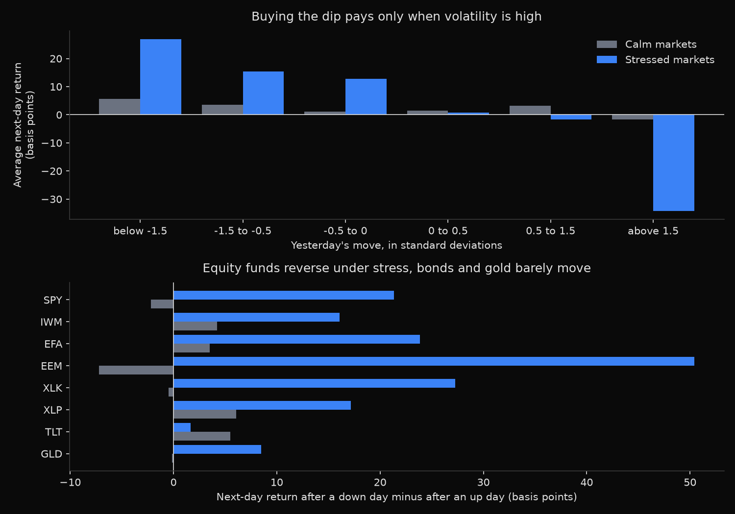
next-day return by the size of yesterday's move (z = return divided by the 20-day standard deviation)
yesterday z      calm days       calm  stressed days   stressed
below -1.5           1,004    5.66 bp          1,015   26.84 bp
-1.5 to -0.5         3,060    3.57 bp          3,038   15.39 bp
-0.5 to 0            2,781    1.14 bp          2,669   12.81 bp
0 to 0.5             2,986    1.43 bp          3,039    0.74 bp
0.5 to 1.5           3,883    3.25 bp          3,627   -1.69 bp
above 1.5            1,146   -1.68 bp            893  -34.17 bp

robustness
first half, 2006-2014                          stressed  28.51 bp (t=2.89)   calm  1.75 bp (t= 0.50)
second half, 2015-2026                         stressed  15.93 bp (t=2.60)   calm  0.48 bp (t= 0.19)
excluding the 2008-09 and 2020 crisis windows  stressed  14.83 bp (t=3.50)   calm  0.74 bp (t= 0.35)

share of next days that close higher
calm      after a down day 54.1%   after an up day 52.1%
normal    after a down day 55.9%   after an up day 52.4%
stressed  after a down day 56.1%   after an up day 51.0%
What this tells us
The reversal spread rises with volatility without a break: 1.05 basis points in calm markets, 7.51 in normal ones, 21.10 under stress. Only the second and third survive a significance test, and the calm figure carries a t-statistic of 0.50 across 14,860 observations. Unconditional dip buying earns nothing.
The effect is two-sided. In stressed markets the day after a rally averages minus 4.67 basis points, against an unconditional average near 4 basis points a day for these funds. Sorting by the size of the move sharpens it: a fall beyond 1.5 standard deviations is followed by 26.84 basis points and a rally of the same size by minus 34.17, a range of 61 basis points. The same cuts in calm markets span 5.66 down to minus 1.68.
Every equity fund reverses more under stress, and emerging markets pay the most at 50.41 basis points, which is what a liquidity premium should look like in the least liquid equity exposure here. Long Treasuries break the pattern in the direction that story predicts, at 1.64 basis points with a t-statistic of 0.29, and gold reaches 8.50, below every equity fund and not significant.
Two checks argue against an artefact. The result holds in both halves of the sample, weakening from 28.51 to 15.93 basis points in the second half, and removing the 2008-09 and 2020 crisis windows still leaves 14.83 basis points at a t-statistic of 3.50.
So what?
Attach a volatility filter to any short-term reversal rule. The signal that returns 21 basis points when 20-day volatility sits in the top third of its two-year range returns 1 basis point in the bottom third.
Size the expectation against the cost: 21 basis points is gross of the round trip on a one-day holding period, which favours the largest and cheapest funds. The emerging markets number is the biggest in the table and the most expensive to capture.
The more durable use is execution rather than strategy. An investor with a purchase already planned gives up little by waiting for the day after a down day when volatility is elevated, and the hit rate of 56.1% against 51.0% says the wait is usually rewarded. The result also carries a warning for daily trend and momentum systems: under stress, yesterday’s direction predicts the reverse of itself, so a rule that buys strength every day trades into that spread rather than earning it.
Built with xfinlink — free financial data API for Python. pip install -U xfinlink
pip install -U xfinlink