
Do Companies That Shrink Their Share Count Outperform? Net Buyback Yield in Python
August 10, 2026
What’s the question?
A buyback announcement authorises spending. It does not commit to it, and it says nothing about what leaves by the other door in stock compensation or shares printed to pay for an acquisition. A company can spend ten billion dollars repurchasing its own stock and finish the year with more shares outstanding than it started with.
Net share-count reduction is the change in shares outstanding between two consecutive annual reports, signed so that shrinking is positive. That is the honest version of buyback yield: everything bought back, less everything issued. Cutting the count lifts every per-share figure mechanically, and a team that keeps cutting is either confident the stock is cheap or short of better uses for cash. If the market is slow to price that, the shrinkers should beat the diluters.
Two things have to be right first. The universe must be the index as it stood on the day, or the result describes companies selected for having survived. And a split multiplies the count without changing anything economic, so a raw ratio reads two-for-one as a 100% dilution.
The approach
The sample is the S&P 500 as it stood on 30 June in each year from 2019 to 2025, seven annual rebalances, with returns measured to the following 30 June. Rosters are read point in time and each company keyed on its entity identifier, because a symbol string is not a company. Data comes from SEC EDGAR filings and market data.
- Take the union of the seven rosters: 619 distinct companies.
- Pull annual shares outstanding and dividends per share, keeping companies whose fiscal year ends in December so every cross-section spans the same twelve months of corporate decisions.
- At each rebalance, use the fiscal years ending the previous December and the December before that, both filed months before the portfolio is formed.
- Correct for splits. Raw closes divided by split-adjusted closes give the cumulative future split factor, so a move in that ratio locates a split and the exact events are read from the price series. Divide it out only where that brings the change into a range a share count can actually move, since some filers restate the earlier count themselves.
- Sort into quintiles and hold each bucket equal weighted for twelve months. A name that stops trading inside the holding year exits at its last clean bar, so acquisitions and failures stay in the sample.
Returns exclude dividends, so each bucket’s trailing yield is reported alongside them.
Code
import numpy as np
import pandas as pd
import xfinlink as xfl

xfl.set_api_key("YOUR_API_KEY")  # free at https://xfinlink.com/signup

YEARS = list(range(2019, 2026))

rosters = {y: xfl.index("sp500", as_of=f"{y}-06-30").dropna(subset=["entity_id"])
                 .astype({"entity_id": int}).set_index("entity_id")["ticker"]
           for y in YEARS + [2026]}
ids = sorted(set().union(*[set(r.index) for r in rosters.values()]))

fu = pd.concat([xfl.fundamentals(entity_id=c, period_type="annual",
                                 start="2016-06-01", end="2025-06-30",
                                 fields=["shares_outstanding", "dividends_per_share"])
                for c in chunked(ids)], ignore_index=True)
pe = fu["period_end"]
fu["fy"] = np.where(pe.dt.month == 1, pe.dt.year - 1, pe.dt.year)
fu = fu[((pe.dt.month == 12) & (pe.dt.day >= 15)) | ((pe.dt.month == 1) & (pe.dt.day <= 15))]

# close / adj_close is the cumulative future split factor. Where it moves between two
# anchor dates, read the exact split events out of that company's daily series.
grid["F"] = grid["close"] / grid["adj_close"]
flag = grid[(grid["F"] / grid.groupby("entity_id")["F"].shift(-1) - 1).abs() > 0.002]
for _, r in flag.iterrows():
    p = xfl.prices(entity_id=int(r["entity_id"]), start=str(r["date"].date()),
                   end=str(r["d_next"].date()), fields=["split_ratio"])
    ev.setdefault(int(r["entity_id"]), []).extend(
        zip(p["date"], p.loc[p["split_ratio"].notna(), "split_ratio"]))

sh = fu.set_index(["entity_id", "fy"])["shares_outstanding"]
for y in YEARS:
    for eid in rosters[y].index:
        raw = sh[(eid, y - 1)] / sh[(eid, y - 2)]      # latest fiscal year over the prior one
        P = split_prod(eid, pe1, pe2 + pd.Timedelta(days=183))
        ratio = raw / P if abs(np.log(raw / P)) < abs(np.log(raw)) - np.log(1.20) else raw
        rows.append((y, eid, 1.0 - ratio))             # positive means the count shrank

sig["fwd"] = sig["px1"] / sig["px0"] - 1               # adj_close at both 30 June anchors
sig["q"] = sig.groupby("year")["reduction"].transform(lambda x: pd.qcut(x, 5, labels=[1, 2, 3, 4, 5]))
print(sig.groupby("q")["fwd"].agg(["size", "mean", "median"]), sig["fwd"].mean())
Full script with formatting and visualisation: net-share-count-reduction-forward-returns-python.py
Output
point-in-time S&P 500 rosters 2019-2026: 619 distinct companies

annual filings with a December fiscal year end: 4005 rows, 471 companies
share-count-changing events found in the price series: 61 across 59 companies

SPLIT AUDIT  (57 company-years had a split near the fiscal year: 34 de-splitted, 23 left alone because the two counts were already on one scale)
   yr ticker     prior (M)   latest (M)      raw    split  signal used
 2019 AFL            390.5        755.3    1.934    2.000        3.28%
 2019 CNC            173.4        412.5    2.378    2.000      -18.91%
 2019 FI             206.6        391.6    1.895    2.000        5.23%
 2019 ROL            218.0        327.3    1.501    1.500       -0.10%
 2020 FAST           285.9        574.1    2.008    2.000       -0.41%
 2019 DD             780.5        784.1    1.005    0.333       -0.47%
 2019 FAST           287.6        285.9    0.994    2.000        0.59%
 2020 CNC            412.5        415.0    1.006    2.000       -0.62%
 2020 DD             784.1        738.6    0.942    0.333        5.81%
 2020 EW             207.7        209.1    1.007    3.000       -0.67%
 2020 ODFL            81.2         79.7    0.981    1.500        1.90%
 2021 APH            297.9        299.3    1.005    2.000       -0.47%
entity-years moving more than 25% before the split adjustment: 87; after: 53

names that stopped trading inside a holding year: 34 (exited at last traded price)
observations dropped by the symbol-integrity check on the two price legs: 28

final panel: 2581 company-years, 352-376 names per rebalance, missing values 0

QUINTILES ON NET SHARE-COUNT REDUCTION, pooled over 7 annual rebalances
bucket                       n  mean signal  mean fwd 1y    median  div yield
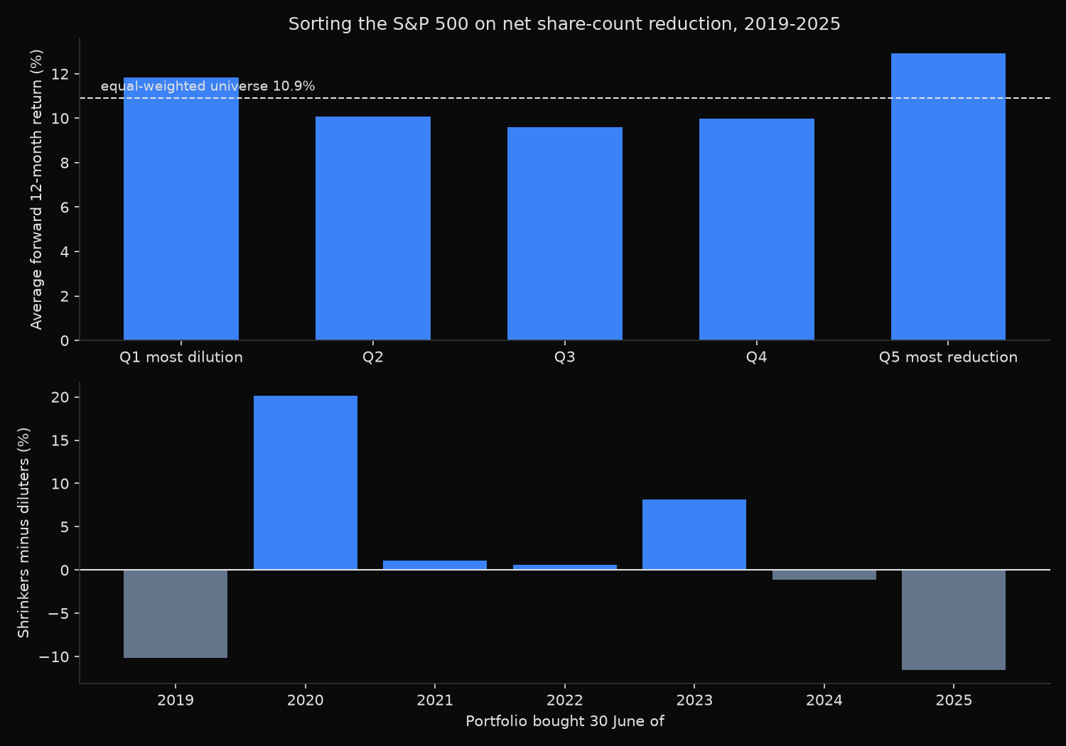
Q1 most dilution           520       -6.02%       11.84%     6.14%      2.07%
Q2                         527       -0.29%       10.06%     6.15%      2.50%
Q3                         502        0.46%        9.60%     5.64%      2.05%
Q4                         514        1.99%        9.99%     6.45%      1.77%
Q5 most reduction          518        6.21%       12.93%     8.47%      1.76%
equal-weighted universe   2581        0.46%       10.89%     6.24%      2.03%

EVERY REBALANCE SEPARATELY (forward 12-month price return, equal weighted)
 buy 30 June        Q1        Q5  universe     Q5-Q1  Q5-universe
        2019    -4.00%   -14.18%    -9.34%   -10.18%       -4.84%
        2020    36.26%    56.40%    46.93%    20.13%        9.46%
        2021   -10.41%    -9.29%    -9.07%     1.12%       -0.22%
        2022     6.82%     7.46%    10.02%     0.64%       -2.57%
        2023     6.06%    14.23%     9.27%     8.16%        4.96%
        2024    17.82%    16.67%    11.00%    -1.15%        5.67%
        2025    30.19%    18.65%    17.18%   -11.55%        1.46%
Q5 beat Q1 in 4 of 7 rebalances; spread mean 1.03%, standard deviation 10.84%, range -11.55% to 20.13%

LARGEST SIGNAL VALUES, checked against the underlying counts
   yr ticker     prior (M)   latest (M)   split  reduction    fwd 1y
 2022 DD             734.2        512.9    1.00     30.14%    28.54%
 2020 DVA            166.4        125.8    1.00     24.37%    52.17%
 2023 MPC            565.2        445.5    1.00     21.17%    48.78%
 2022 WTW            129.0        102.5    1.00     20.54%    19.31%
 2024 EXR            133.9        211.3    1.00    -57.76%    -5.13%
 2023 VICI           628.9        963.1    1.00    -53.13%    -8.88%
 2019 CI             250.9        380.9    1.00    -51.83%    19.11%
 2020 NEM            533.0        808.0    1.00    -51.59%     2.66%
What this tells us
The shrinkers did beat the index. Q5 averaged 12.93% over the following twelve months against 10.89% for the equal-weighted universe, and the gap is wider on the median, 8.47% against 6.24%, so it does not rest on a few large winners.
The long-short version does not work. Q5 beat Q1 by 1.03 points on average with a standard deviation of 10.84 points, and the years run from minus 11.55% to plus 20.13%. Seven observations with that much scatter cannot separate a one-point edge from zero. The signal also failed where it should have helped most: the 2019 portfolio, held through the pandemic crash, lost 14.18% against the index’s 9.34%, because the companies retiring stock held the least cash when revenue stopped.
What kills the trade is that the relationship is not monotone. The heaviest diluters returned 11.84%, ahead of all three middle buckets, so both ends of the sort beat the centre. The extremes explain why: Extra Space Storage issued 58% more shares for Life Storage, VICI 53% more for MGM Growth Properties, Cigna for Express Scripts, Newmont for Goldcorp. Large-cap dilution is mostly acquisition currency rather than distress, and the market prices those deals on their merits. Dividends tilt the comparison slightly toward the shrinkers, whose 1.76% trailing yield sits below the diluters’ 2.07%.
The split audit shows how much of this is measurement rather than economics. Before the correction, 87 company-years appeared to move their count by more than 25%; afterwards 53 did, and every one is a merger, a separation, or an enormous repurchase programme.
So what?
Use net share-count reduction as a quality filter, not as a factor. A fifth of the index earning two points a year above it is worth having inside a screen that already selects on something else, and the median says the effect reaches the typical name. Nothing here supports a long-short book: a one-point spread with an eleven-point standard deviation is a coin flip carrying a borrow cost.
Read the sign before acting on it, because dilution and repurchase are not opposites. Separate the diluters issuing stock to buy a business from those issuing because they need the money; the two behave nothing alike, and lumping them together flattens the bottom of the sort.
For any company whose buyback is part of the investment case, check the count against the announcement: two annual filings and one split adjustment measure what was actually delivered.
Built with xfinlink — free financial data API for Python. pip install -U xfinlink
pip install -U xfinlink