
What If You Miss the Market's Best Days? Extreme-Day Analysis in Python
August 7, 2026
What’s the question?
Every argument against market timing eventually reaches the same statistic: miss the ten best days and most of your return disappears. It appears in fund brochures, advisor presentations, and roughly every article written about staying invested. The number is arithmetically correct.
What makes it persuasive is an unstated assumption. The statistic only supports “never sell” if the best days are scattered unpredictably through calm markets, so that any exit carries a real chance of missing one. Presented that way, the reader concludes that timing is a lottery with terrible odds.
The same calculation run in the other direction is almost never shown. If a handful of days determines the outcome, then missing the ten worst days should matter about as much, and in the opposite direction. Whether the one-sided version is a fair summary depends entirely on where in the historical record these extreme days actually sit.
The approach
The test uses four funds covering US large caps, US small caps, developed international markets, and emerging markets, on daily total returns from 1996 to the end of 2024. SPY alone contributes 7,300 sessions.
- Compute the annual compound return with every session included.
- Remove the 10, 20, and 30 largest single-day gains and recompute. A removed day is treated as a flat session rather than as a shortened history, which is what being out of the market for that day would mean.
- Repeat, removing the largest single-day losses instead.
- Repeat again, removing both tails at once.
- Measure how far each of the 20 best days sits from the nearest of the 20 worst, counted in trading sessions, and tabulate which calendar years hold them.
The fourth step carries the argument. Any rule that takes an investor out of the market for a stretch removes whatever falls inside that stretch, gains and losses together, so the paired removal is the only one that resembles what timing actually does.
Code
import pandas as pd
import xfinlink as xfl

xfl.set_api_key("YOUR_API_KEY")  # free at https://xfinlink.com/signup

d = xfl.prices("SPY", start="1996-01-01", end="2024-12-31",
               fields=["close", "return_daily"]).sort_values("date")
d["date"] = pd.to_datetime(d["date"])
r = d.dropna(subset=["return_daily"]).set_index("date")["return_daily"]

def cagr(x):
    yrs = (x.index[-1] - x.index[0]).days / 365.25
    return ((1 + x).prod() ** (1 / yrs) - 1) * 100

def drop(x, n, which):
    o = x.sort_values()
    kill = {"best": o.index[-n:], "worst": o.index[:n],
            "both": o.index[-n:].union(o.index[:n])}[which]
    return x.drop(kill)

print(f"all in           {cagr(r):.2f}%")
for n in (10, 20, 30):
    print(f"-{n:2d} best  {cagr(drop(r, n, 'best')):6.2f}%   "
          f"-{n:2d} worst {cagr(drop(r, n, 'worst')):6.2f}%   "
          f"-{n:2d} both  {cagr(drop(r, n, 'both')):6.2f}%")
Full script with formatting and visualisation: missing-best-worst-days-market-timing-python.py
Output
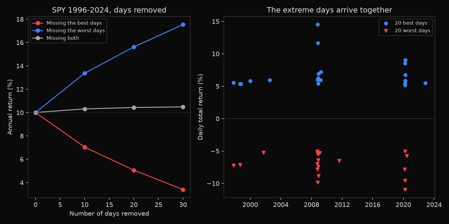
Daily total returns, 1996-01-01 to 2024-12-31
     exposure          days  all in  -10 best  -10 worst  -10 both
SPY  US large cap      7300  10.01%     7.04%     13.37%    10.32%
IWM  US small cap      6187   8.02%     4.81%     12.50%     9.16%
EFA  Developed intl    5878   5.30%     1.55%      9.63%     5.73%
EEM  Emerging mkts     5467   8.35%     2.35%     14.45%     8.11%

SPY only, deeper cuts
  removed     best    worst     both
        0   10.01%   10.01%   10.01%
       10    7.04%   13.37%   10.32%
       20    5.07%   15.62%   10.43%
       30    3.41%   17.54%   10.49%

20 best days: median 4 sessions from the nearest of the 20 worst; 12 of 20 within a week, 14 within a month
best-20 by year:  1997:1, 1998:2, 2000:1, 2002:1, 2008:6, 2009:2, 2020:6, 2022:1
worst-20 by year: 1997:1, 1998:1, 2001:1, 2008:10, 2009:1, 2011:1, 2020:5
years holding both a best-20 and a worst-20 day: [1997, 1998, 2008, 2009, 2020] (85% of best days)

the five largest single-session gains and what preceded them
  2008-10-13  +14.52%   prior 5 sessions  -19.79%
  2008-10-28  +11.69%   prior 5 sessions  -15.04%
  2020-03-24  + 9.06%   prior 5 sessions   -6.48%
  2020-03-13  + 8.55%   prior 5 sessions  -17.97%
  2009-03-23  + 7.18%   prior 5 sessions    1.55%
What this tells us
The headline statistic survives contact with the data. Ten sessions out of 7,300, fourteen hundredths of one percent of the sample, carry roughly three percentage points of annual return. Remove thirty and SPY falls from 10.01% to 3.41%. Emerging markets are more extreme still, dropping from 8.35% to 2.35% on ten days.
The mirror image is equally strong and rarely quoted. Missing the worst ten days lifts SPY to 13.37%, and the worst thirty lifts it to 17.54%. Both columns come from the same property of the return distribution: a small number of sessions dominates the compound outcome. Only one of them ever appears in the brochure.
Removing both tails settles the question. SPY returns 10.32% without its best and worst ten days, 10.43% without twenty of each, and 10.49% without thirty, against 10.01% with everything included. The two tails cancel almost exactly, and the slight edge to the trimmed version comes from the reduced volatility drag of a narrower distribution.
The clustering explains why. The median gap between one of the 20 best days and the nearest of the 20 worst is 4 trading sessions, and 12 of the 20 best days fall within a single week of a worst day. The years holding the best days are the years holding the worst: 2008 contributes 6 of the best and 10 of the worst, and 2020 contributes 6 and 5. Across the full sample, 85% of the best days landed in a year that also produced one of the worst.
The largest gains make the mechanism concrete. SPY rose 14.52% on 13 October 2008, immediately after losing 19.79% over the previous five sessions, and 8.55% on 13 March 2020 after a 17.97% five-session decline. The best days are not scattered through calm markets at all. They are rebounds inside crashes, and an investor positioned to miss them was almost certainly positioned to miss the collapse that produced them.
So what?
The statistic is a sound argument against one specific mistake: selling in a panic and returning only once the recovery is visible. That sequence really does capture the losses and forfeit the rebounds, and it is the most common way retail investors damage a portfolio.
It is not a general argument against every timing rule, and it is often used as one. A rule that reduces exposure through a turbulent stretch removes days from both tails, and the paired-removal column shows that trade is close to neutral on return while cutting the range of outcomes considerably. Judging such a rule by the best-days number alone assumes it will catch the rebounds while somehow sitting through the collapse, which is not a description of any mechanical strategy.
Use this as a template for evaluating any timing proposal. Ask what it does to both tails rather than one, and quote both columns whenever the best-days figure is cited. When someone presents the one-sided version, the missing column is not a detail: it points the opposite way and is the same size.
Built with xfinlink — free financial data API for Python. pip install -U xfinlink
pip install -U xfinlink