
Does Trend Following Beat Buy and Hold? Time-Series Momentum in Python
August 1, 2026
What’s the question?
Time-series momentum, usually called trend following, is the claim that an asset’s own recent return predicts its next one. It differs from the cross-sectional momentum most factor research studies, which ranks assets against each other and buys the winners. Here the comparison is only against zero: if gold rose over the past year, hold gold; if it fell, do not.
The claim has two halves that often get collapsed into one. The first is statistical: does the sign of a trailing return carry information about next month’s return? The second is economic: does acting on that sign deliver more return per unit of risk than holding the asset outright? A rule can fail the first and pass the second, because stepping into cash during a decline reshapes the return distribution even when nothing was forecast.
The approach
Eleven liquid funds cover US large and small cap equity, developed and emerging international equity, listed real estate, Treasuries at two maturities, investment grade and high yield credit, gold and broad commodities. Treasury bills (BIL) are the cash leg, so capital stepping out earns the bill rate rather than zero.
- Pull daily total returns from June 2007 and compound them into calendar-month returns.
- At each month end, compute every asset’s own trailing k-month return for k of 1, 3, 6, 9 and 12 months.
- Hold the asset through the following month when that return is positive, hold bills otherwise. The signal uses data through month t-1 and the position runs during month t, so no future information enters.
- Test predictability separately: each month, subtract the average excess return of the negative-signal assets from that of the positive-signal assets, then t-test that monthly series.
- Compare annualised return, volatility, Sharpe and maximum drawdown against buy-and-hold, and test each Sharpe difference with the Memmel-corrected Jobson-Korkie statistic.
All five lookbacks run over the same 218 months from June 2008, since the 12-month signal needs a year of history first.
Code
import numpy as np
import pandas as pd
from scipy import stats
import xfinlink as xfl

xfl.set_api_key("YOUR_API_KEY")  # free at https://xfinlink.com/signup

ASSETS = ["SPY", "IWM", "EFA", "EEM", "VNQ", "TLT", "IEF", "LQD", "HYG", "GLD", "DBC"]
LOOKBACKS = [1, 3, 6, 9, 12]

px = pd.concat(
    [xfl.prices(t, start="2007-06-01", fields=["return_daily"]) for t in ASSETS + ["BIL"]]
)
daily = px.pivot_table(index="date", columns="ticker", values="return_daily")
monthly = ((1 + daily).resample("ME").prod() - 1)["2007-06-30":]
rf, R = monthly["BIL"], monthly[ASSETS]

win = R.index >= R.index[max(LOOKBACKS)]     # common window for every lookback
rf_w = rf[win]
bh = R[win].mean(axis=1)                     # equal-weight buy-and-hold

signal = {k: (((1 + R).rolling(k).apply(np.prod, raw=True) - 1) > 0).astype(float)
          for k in LOOKBACKS}

excess = R[win].sub(rf_w, axis=0)
for k in LOOKBACKS:
    s = signal[k].shift(1)[win]              # signal from month t-1, held in month t
    up, dn = excess.where(s == 1).mean(axis=1), excess.where(s == 0).mean(axis=1)
    diff = (up - dn)[up.notna() & dn.notna()]
    t, p = stats.ttest_1samp(diff, 0)

    port = (R[win] * s + rf_w.values[:, None] * (1 - s)).mean(axis=1)
    ex = port - rf_w
    eq = (1 + port).cumprod()
    print(f"{k:2d}m  spread {diff.mean()*100:+.3f}%/mo (t {t:+.2f}, p {p:.3f})  "
          f"return {((1+port).prod()**(12/len(port))-1)*100:.2f}%  "
          f"Sharpe {ex.mean()/ex.std(ddof=1)*np.sqrt(12):.2f}  "
          f"maxDD {(eq/eq.cummax()-1).min()*100:.2f}%")
Full script with formatting and visualisation: time-series-momentum-trend-following-python.py
Output
Sample        : 2007-06-30 to 2026-07-31 monthly, 11 assets, cash leg BIL
Backtest      : 2008-06-30 to 2026-07-31  (218 months)

Next-month excess return, sorted on the sign of the trailing k-month return
 lookback   obs +   obs -   mean +   mean -   spread      t      p   hit +   hit -
       1m    1374    1024  +0.619%  +0.327%  +0.291%  +0.98  0.331   55.5%   56.2%
       3m    1497     901  +0.631%  +0.456%  +0.175%  +0.54  0.588   57.4%   53.2%
       6m    1579     819  +0.468%  +0.347%  +0.121%  +0.42  0.678   56.8%   53.8%
       9m    1573     825  +0.413%  +0.090%  +0.322%  +1.13  0.262   56.8%   53.9%
      12m    1622     776  +0.425%  +0.286%  +0.139%  +0.49  0.624   56.8%   53.6%
         unconditional mean +0.429% per month, hit rate 55.8%

Equal-weight composite: long/flat trend rule vs buy-and-hold
                return     vol  Sharpe   max DD  switches/yr   JK z      p
buy-and-hold     5.96%  10.90%    0.47  -30.55%         0.00
trend 1m         3.92%   5.89%    0.47  -15.54%         5.81  -0.02  0.981
trend 3m         5.15%   5.95%    0.66   -8.88%         2.81  +1.00  0.319
trend 6m         5.07%   5.94%    0.65   -7.00%         1.90  +1.07  0.286
trend 9m         4.28%   6.10%    0.51  -10.17%         1.66  +0.24  0.809
trend 12m        4.83%   6.14%    0.59   -9.11%         1.28  +0.73  0.464

Per asset, 12-month rule
                        B&H ret  B&H Sh   B&H DD  trend ret  trend Sh  trend DD  invested
SPY  US large cap        11.58%    0.70  -41.81%     10.80%      0.79   -19.44%     83.9%
IWM  US small cap         9.26%    0.47  -46.48%      5.58%      0.37   -32.68%     69.3%
EFA  Developed ex-US      4.85%    0.29  -48.85%      2.43%      0.16   -36.49%     63.3%
EEM  Emerging markets     3.49%    0.21  -52.41%      3.77%      0.25   -32.91%     60.1%
VNQ  REITs                6.23%    0.33  -59.70%      4.87%      0.32   -27.33%     70.6%
TLT  Long Treasuries      2.52%    0.16  -47.61%      2.47%      0.16   -24.85%     59.2%
IEF  7-10yr Treasuries    2.48%    0.21  -23.15%      3.11%      0.36    -8.48%     64.7%
LQD  IG credit            4.08%    0.37  -23.27%      3.61%      0.39   -12.27%     78.4%
HYG  High yield           5.13%    0.41  -27.19%      3.40%      0.40   -12.99%     80.3%
GLD  Gold                 8.29%    0.48  -42.91%      6.75%      0.43   -28.95%     65.6%
DBC  Commodities         -0.93%   -0.02  -74.54%      0.87%      0.05   -49.24%     48.6%

Crisis window 2008-06-30 to 2009-12-31: buy-and-hold -5.32%, trend 1m +9.63%, trend 3m +11.53%, trend 6m +11.26%, trend 9m +2.42%, trend 12m +2.48%
From 2010-01 onward (199 months): buy-and-hold Sharpe 0.62, max DD -19.47%; trend 1m Sharpe 0.48, trend 3m Sharpe 0.66, trend 6m Sharpe 0.64, trend 9m Sharpe 0.57, trend 12m Sharpe 0.64
What this tells us
The predictability test finds nothing at any horizon. Spreads run from +0.121 percent per month at six months to +0.322 percent at nine months, with t-statistics between +0.42 and +1.13 and p-values no lower than 0.262. Hit rates say it plainly: assets flagged positive by the 12-month signal produced a positive excess return 56.8 percent of the time against 53.6 percent for those flagged negative, on an unconditional rate of 55.8 percent across all 2,398 asset-months.
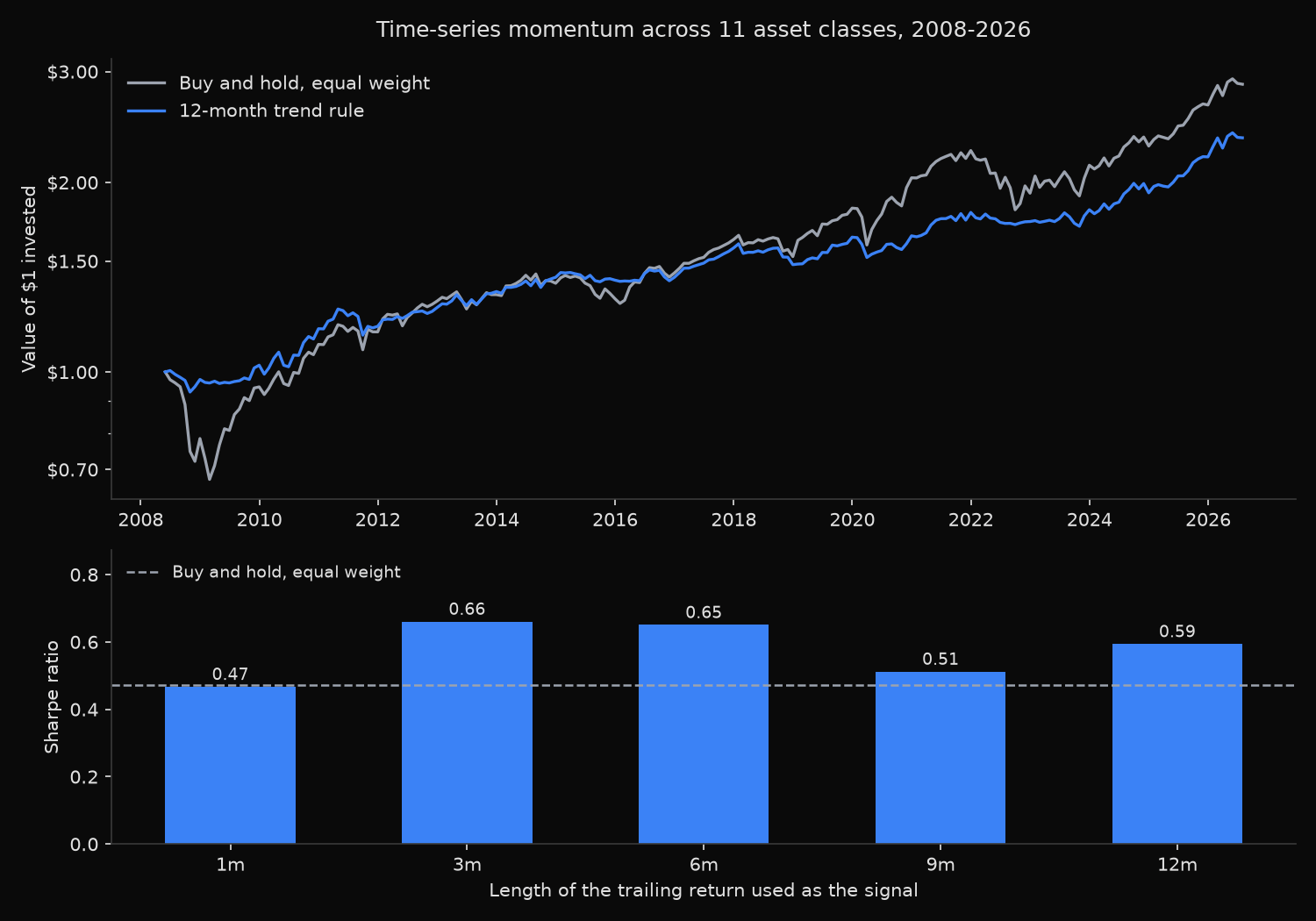
The backtest reads as a contradiction until the mechanism is separated out. Composite volatility falls from 10.90 percent to roughly 6, maximum drawdown from 30.55 percent to between 7.00 and 15.54, and Sharpe clears buy-and-hold at four of the five horizons, peaking at 0.66 against 0.47. None of those gaps is significant, the largest Jobson-Korkie statistic being z of +1.07 at p of 0.286.
Return falls at every horizon, from 5.96 percent to between 3.92 and 5.15, which is arithmetic, not bad luck: the 12-month rule holds the risky asset only 67.6 percent of the time, and bills compounded at 1.27 percent a year. The rule does not earn its risk reduction, it buys it by sitting out.
What remains concentrates in one episode. Between June 2008 and December 2009 buy-and-hold lost 5.32 percent while the trend rule gained 2.42 to 11.53 percent. Remove those nineteen months and buy-and-hold’s Sharpe climbs to 0.62 against 0.64 for the 12-month rule, which beat it in only 39 percent of individual months.
So what?
Trading costs are not the obstacle. The 12-month rule switches position 1.28 times per asset-year, so at 5 basis points a trade the drag is about 6 basis points a year, and even the twitchy one-month rule at 5.81 switches costs roughly 29 basis points against a return gap of 113. Turnover is not what separates the two lines.
Read the rule as a risk-shaping tool, not a forecast. Where the binding constraint is drawdown tolerance, cutting the worst peak-to-trough loss from 30 percent to 9 in exchange for 113 basis points a year is a reasonable trade. Where the purchase is predicted return, the evidence here does not support it.
Two checks are worth running before committing capital. Re-estimate with the crisis window excluded, since that is where the edge lived. Then note how flat the horizon grid is: Sharpes of 0.47, 0.66, 0.65, 0.51 and 0.59 over identical months. Picking the winner from a grid that tight is curve fitting, so a live allocation should assume the middle of the range rather than the top.
Built with xfinlink — free financial data API for Python. pip install -U xfinlink
pip install -U xfinlink