Can Anything Predict Next Month's Stock Returns? Out-of-Sample R-Squared Testing in Python

August 9, 2026

What’s the question?

Every forecast of the stock market competes with a rival that needs no model: the average return so far. If the market has delivered roughly 0.9% a month since the data began, then “0.9% next month” is a forecast, and it costs nothing to produce.

Welch and Goyal put that comparison on the record in 2008. They regenerated the standard predictors of the equity premium using only the data an investor would have had at the time, and found that almost none beat the running historical average. A regression fitted on the full history has already seen the answers, including the crash nobody saw coming; a live forecast comes out of data ending the day before.

The measure of the gap is the out-of-sample R-squared: one minus the ratio of the model’s squared forecast errors to those of the prevailing mean, which is the running average of every month up to that point. Above zero the model beat the average. Campbell and Thompson (2008) added a refinement that matters here. When a model forecasts a negative expected return for equities, override it with zero, since no investor rationally holds stocks while expecting to lose money.

The approach

The target is the monthly total return on SPY. Every predictor is built from exchange-traded fund prices, so each input is observable on the last day of the month it belongs to.

1. Compound daily total returns into calendar-month returns for SPY, MDY, TLT, SHY, LQD and IEF, from July 2002 through July 2026.
2. Form five predictors: the trailing 12-month return on SPY (momentum), the annualised standard deviation of the last 12 monthly returns (volatility), TLT minus SHY over 12 months (a term spread proxy), LQD minus IEF (a credit spread proxy, investment-grade corporates against Treasuries of similar duration), and MDY minus SPY (a size spread).
3. Fit each predictive regression on an expanding window of at least 60 months, forecast the next month, add the realised observation and refit. A sixth model uses all five predictors at once.
4. Score every forecast against the prevailing mean, then repeat with the Campbell-Thompson restriction.

The bond pairs are return spreads rather than yield spreads; a widening spread shows up as one leg outperforming the other. The restriction applies to the total return rather than the excess return over cash, making it a slightly weaker version of the original. That leaves 216 live forecasts covering August 2008 through July 2026, a window that opens in the middle of the financial crisis.

Code

import numpy as np
import pandas as pd
import xfinlink as xfl

xfl.set_api_key("YOUR_API_KEY")  # free at https://xfinlink.com/signup

px = xfl.prices(["SPY", "MDY", "TLT", "SHY", "LQD", "IEF"],
                start="2002-07-01", end="2026-07-31",
                fields=["return_daily"], max_rows=200000)
px = px.dropna(subset=["return_daily"])
px["month"] = px["date"].dt.to_period("M")

monthly = (px.groupby(["ticker", "month"])["return_daily"]
             .apply(lambda r: (1.0 + r).prod() - 1.0).unstack(0).sort_index().iloc[1:])

t12 = lambda c: (1.0 + monthly[c]).rolling(12).apply(np.prod, raw=True) - 1.0
data = pd.DataFrame({
    "momentum": t12("SPY"),
    "volatility": monthly["SPY"].rolling(12).std() * np.sqrt(12),
    "term spread": t12("TLT") - t12("SHY"),
    "credit spread": t12("LQD") - t12("IEF"),
    "size spread": t12("MDY") - t12("SPY"),
    "y_next": monthly["SPY"].shift(-1),
}).dropna()

y = data["y_next"].to_numpy()
MIN_TRAIN, n = 60, len(data)

for cols in [["momentum"], ["volatility"], ["term spread"],
             ["credit spread"], ["size spread"],
             ["momentum", "volatility", "term spread", "credit spread", "size spread"]]:
    x = data[cols].to_numpy()
    fcst, mean_fcst = np.full(n, np.nan), np.full(n, np.nan)
    for i in range(MIN_TRAIN, n):
        A = np.column_stack([np.ones(i), x[:i]])
        beta = np.linalg.lstsq(A, y[:i], rcond=None)[0]
        fcst[i] = beta[0] + np.dot(beta[1:], x[i])
        mean_fcst[i] = y[:i].mean()

    live = slice(MIN_TRAIN, n)
    sse_mean = np.sum((y[live] - mean_fcst[live]) ** 2)
    oos = 1.0 - np.sum((y[live] - fcst[live]) ** 2) / sse_mean
    oos_ct = 1.0 - np.sum((y[live] - np.maximum(fcst[live], 0.0)) ** 2) / sse_mean
    print(f"{'+'.join(cols):20} OOS R2 {oos * 100:6.2f}%   restricted {oos_ct * 100:6.2f}%")

Full script with formatting and visualisation: out-of-sample-return-predictability-python.py

Output

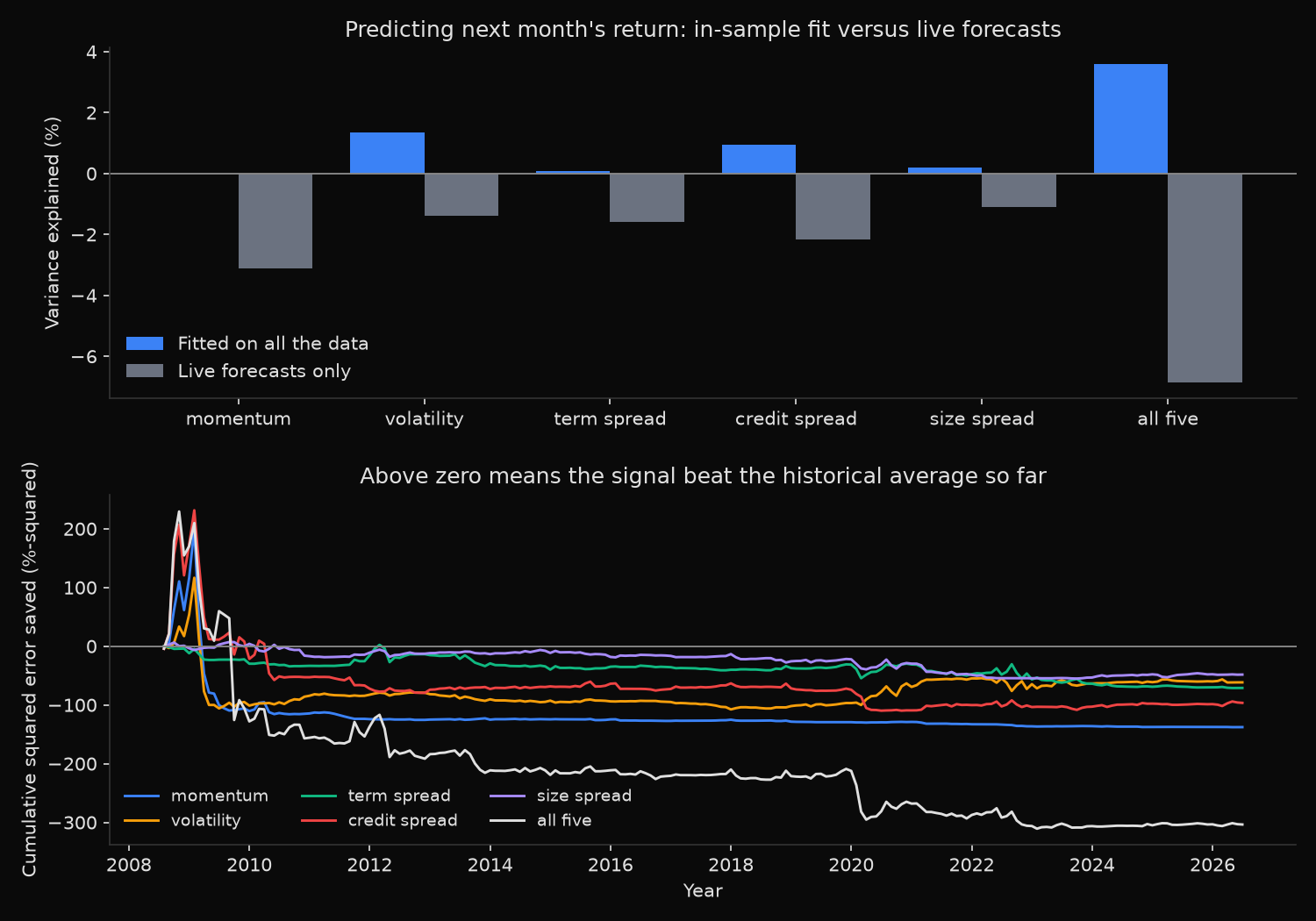
Forecasting SPY monthly total return, one month ahead
Training starts 2003-07, 216 live forecasts 2008-08 to 2026-07

model             in-sample R2   OOS R2  OOS R2 (CT)  sign hit%
momentum                 0.00%   -3.11%       -0.13%      66.7%
volatility               1.34%   -1.39%        1.23%      67.1%
term spread              0.07%   -1.60%       -1.13%      65.3%
credit spread            0.94%   -2.18%       -1.53%      65.7%
size spread              0.20%   -1.09%       -0.78%      64.4%
all five                 3.61%   -6.85%       -5.84%      64.4%

Benchmark: prevailing mean of 0.60% at the first forecast, 0.97% at the last
Realised mean over the live window: 1.07% per month, standard deviation 4.52%
Positive months in the live window: 67.6% (the base rate the sign hit rate has to beat)
Best out-of-sample model: size spread at -1.09%

What this tells us

Every unrestricted model loses to the prevailing mean, from -1.09% for the size spread to -6.85% for all five together. The combination is the most instructive row: fitted on the whole sample it explains 3.61% of the variance in next-month returns, more than double the best single predictor, and that is the number a careless research process would report. Its live forecasts are the worst of the six. Five coefficients estimated on a few dozen noisy observations fit the sample’s accidents, and the accidents do not repeat.

Truncating negative forecasts to zero lifts momentum from -3.11% to -0.13% and turns volatility from -1.39% into +1.23%. The restriction only changes months where the model called a decline, so its entire effect comes from suppressing bearish forecasts that were wrong. Volatility is the one signal carrying real information: high trailing volatility predicts lower forward returns, and once the estimate cannot swing to an implausible negative, what remains beats the historical average. A monthly out-of-sample R-squared above 1% is economically meaningful at that frequency, on one asset and one sample.

The sign hit rates deserve suspicion rather than credit. They cluster between 64.4% and 67.1%, which reads well until the base rate appears: 67.6% of months in the window were positive. A forecast that always said “up” would have scored 67.6%, better than every model in the table. Directional accuracy on an asset with a strong upward drift measures the drift.

So what?

Build the prevailing mean into the evaluation before building the model. Any predictive regression should report an out-of-sample R-squared against a running historical average, and a signal that cannot clear zero describes the past rather than forecasting the future.

Where a signal does survive, restrict it. Truncating implausible forecasts takes one line of code and improved all six models here, because unconstrained regressions produce extreme predictions exactly when the training window holds an unusual episode.

What survives supports position sizing, not direction. An out-of-sample R-squared a little above 1% justifies trimming exposure when trailing volatility is high and justifies nothing in the way of monthly timing calls. A strategy that needs a reliable view of next month’s direction rests on the row reading -6.85%.

Built with xfinlink — free financial data API for Python. pip install -U xfinlink