
Does Past Beta Predict Future Beta? Beta Stability Testing in Python
August 8, 2026
What’s the question?
Beta measures how much a stock moves for each point the market moves, and it is estimated from history. Every use of it is a forecast: position sizing, hedge ratios, and risk models all apply a number fitted on past returns to a future the data has not seen. That step is rarely tested.
Marshall Blume showed in “Betas and Their Regression Tendencies” (Journal of Finance, 1975) that estimated betas drift toward one over successive periods. The practitioner response is the adjusted beta reported by Bloomberg, which fixes the correction at two thirds weight on the regression estimate and one third on 1.00, regardless of stock or period.
Two things follow that a user of adjusted beta should want checked: how much of the ranking survives into the next period, and whether a fixed two-thirds shrinkage suits a recent sample.
The approach
The cross-section must be chosen before any of the returns it is measured on, or the sample quietly excludes companies that failed or were acquired, which are exactly the ones whose betas moved most.
- Take the S&P 500 membership as it stood on 31 December 2015, then keep every third company in entity order. The sample is fixed in 2015 and the sort is unrelated to beta.
- Pull weekly returns from 2016 through 2025, keyed on the company identifier rather than the ticker string, so a company that changed symbol inside the window keeps one continuous series instead of splitting into two partial ones.
- Estimate each company’s beta against SPY by ordinary least squares in five consecutive two-year windows, requiring at least 80 weekly observations in a window.
- Pair each window with the one after it, then measure the cross-sectional correlation, fit the regression of realised beta on prior beta, and compare forecast errors for four rules.
Weekly returns rather than daily is the standard choice for a two-year beta: 104 observations per window, with less of the non-synchronous trading noise that inflates daily estimates.
Code
import numpy as np
import pandas as pd
import xfinlink as xfl

xfl.set_api_key("YOUR_API_KEY")  # free at https://xfinlink.com/signup

members = xfl.index("sp500", as_of="2015-12-31")
ids = sorted(members["entity_id"].dropna().astype(int).unique())
sample = ids[::3]

px = xfl.prices(entity_id=sample, start="2016-01-01", end="2025-12-31",
                interval="1w", fields=["close", "return_daily"], max_rows=200000)
spy = xfl.prices("SPY", start="2016-01-01", end="2025-12-31",
                 interval="1w", fields=["close", "return_daily"])
px["date"] = pd.to_datetime(px["date"])
spy["date"] = pd.to_datetime(spy["date"])
wk = px.pivot_table(index="date", columns="entity_id", values="return_daily")
mkt = spy.set_index("date")["return_daily"].reindex(wk.index)

def betas(y0, y1, min_obs=80):
    m = mkt[str(y0):str(y1)]
    out = {}
    for t in wk.columns:
        r = wk[t].loc[m.index]
        ok = r.notna() & m.notna()
        if ok.sum() >= min_obs:
            out[t] = np.polyfit(m[ok], r[ok], 1)[0]
    return pd.Series(out)

est = pd.DataFrame({f"{a}-{b}": betas(a, b)
                    for a, b in [(2016, 2017), (2018, 2019), (2020, 2021),
                                 (2022, 2023), (2024, 2025)]})
Full script with formatting and visualisation: does-past-beta-predict-future-beta-python.py
Output
495 members at 2015-12-31, systematic sample of 165
523 weeks, 164 companies with a weekly record

window        names    mean  median      sd     min     max
2016-2017       152    1.09    1.08    0.50   -0.63    2.35
2018-2019       145    1.00    1.02    0.35    0.17    1.88
2020-2021       141    1.18    1.16    0.53   -0.71    2.69
2022-2023       137    0.97    0.99    0.38    0.17    1.94
2024-2025       133    0.80    0.78    0.51   -0.11    2.34

from         to               n    corr   slope  intercept
2016-2017    2018-2019      145   0.705   0.482      0.466
2018-2019    2020-2021      140   0.404   0.606      0.574
2020-2021    2022-2023      137   0.439   0.312      0.606
2022-2023    2024-2025      133   0.723   1.012     -0.171

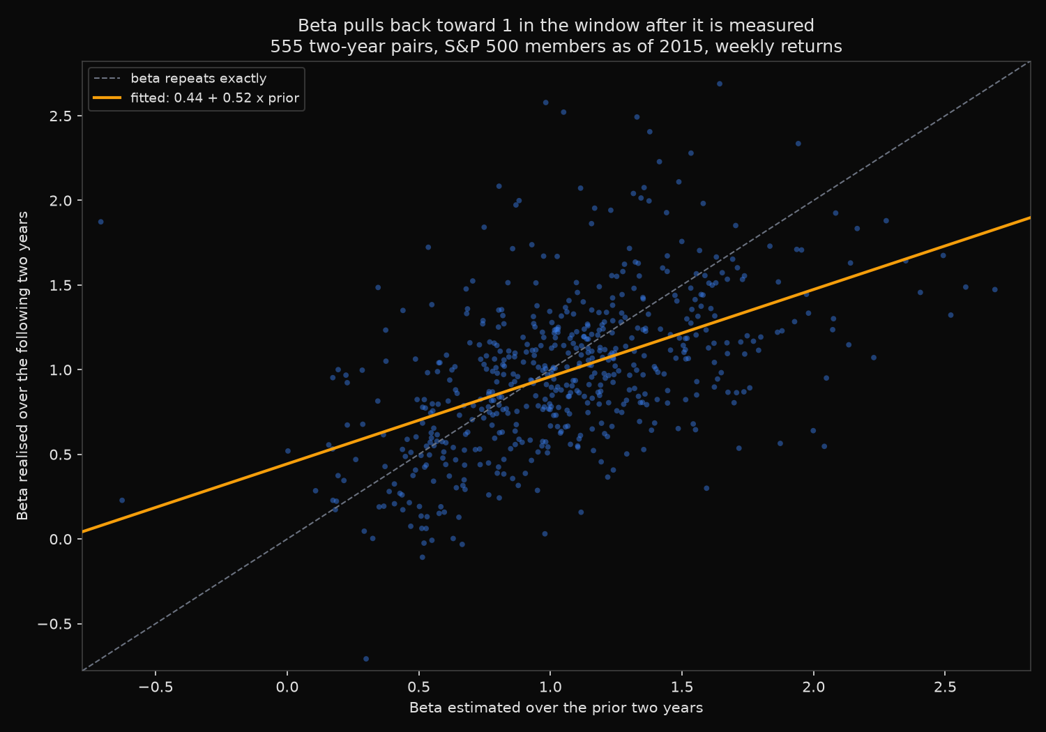
pooled: n=555  corr=0.502  next = 0.444 + 0.515 x prior
Bloomberg's standard adjustment is a fixed 0.67 x prior + 0.33

forecast                       MAE    RMSE    bias
raw prior beta               0.350   0.464   0.069
Bloomberg 0.67b + 0.33       0.313   0.412   0.050
fitted on this sample        0.304   0.403   0.000
always 1.00                  0.358   0.466   0.011

quintile      n  mean prior  mean next    drift
1           111        0.45       0.55    +0.10
2           111        0.82       0.95    +0.13
3           111        1.05       1.00    -0.04
4           111        1.26       1.14    -0.12
5           111        1.72       1.31    -0.41
What this tells us
Pooled across 555 pairs, the correlation between a company’s beta in one two-year window and the next is 0.502. Squared, that is about a quarter of the variation in the next period’s beta explained by the current estimate. Beta carries real information about the future, and considerably less than the precision of the estimate suggests.
Persistence is not stable across regimes. The two transitions that skip the pandemic (0.705 and 0.723) hold roughly twice the correlation of the two that include it (0.404 and 0.439). A period in which every stock’s relationship to the market was rewritten leaves prior betas close to uninformative.
The fitted regression is flatter than the standard adjustment. On this sample the realised beta is 0.444 plus 0.515 times the prior estimate, against Bloomberg’s fixed 0.67 slope. Betas over 2016 to 2025 regressed toward the mean harder than the conventional rule assumes, and the forecast errors follow: mean absolute error of 0.350 using the raw estimate, 0.313 with the Bloomberg adjustment, and 0.304 with the slope fitted on the sample itself. The Bloomberg rule captures most of the available improvement without being fitted to the data at all. That the raw estimate still beats assuming beta equals one for everybody (0.358) matters too, thinly but definitely: the ranking is worth something rather than nothing.
Drift concentrates in the extremes and is asymmetric: the top quintile averaged 1.72 and came back to 1.31, while the bottom rose only 0.10 from 0.45. Middle quintiles barely move. Two estimates show why the tails are unreliable, Newmont at -0.63 over 2016-2017 and GameStop at -0.71 over 2020-2021, when a short squeeze made its returns unrelated to anything the market was doing.
So what?
Shrink extreme betas before using them, and shrink them harder than the standard rule. A hedge ratio built on a raw estimate of 1.7 is sizing against an exposure that historically arrived closer to 1.3. The Bloomberg adjustment captures most of that correction and is the sensible default; fitting the slope on a recent sample adds a further improvement worth having on large positions.
Treat the middle differently from the tails. Companies whose beta sits between roughly 0.8 and 1.3 drift by less than 0.15 on average, so the estimate can be used close to raw. The correction earns its keep at the extremes.
Re-estimate after any period that reprices market-wide relationships, rather than on a calendar. The correlation halved across windows containing 2020, so a model refreshed annually would have carried pre-pandemic betas into a market where they no longer applied. Running this test on a specific universe takes one price pull: a persistence correlation near 0.7 justifies a light adjustment, and one near 0.4 argues for shrinking most of the way to one.
Built with xfinlink — free financial data API for Python. pip install -U xfinlink
pip install -U xfinlink