
Do Low-Volatility Stocks Deliver Better Risk-Adjusted Returns? S&P 500 Quintile Sorts in Python
August 1, 2026
What's the question?
Finance theory prices risk: take more of it, and the market is supposed to pay for it. Equity markets have declined to cooperate for half a century. Fischer Black documented a flat beta-to-return relationship in 1972, and Baker, Bradley and Wurgler reported in 2011 that the least volatile US stocks had beaten the most volatile over four decades.
Two claims travel under the name “low-volatility anomaly”. The strong one says calm stocks earn more outright; the weak one says they earn less but carry so much less risk that return per unit of risk still favours them. Low-volatility funds are sold on the strong claim and defended on the weak one.
Which survives a mechanical test on the S&P 500 over the past decade?
The approach
The universe is the S&P 500 as it stood at each formation date, not as it stands today. That choice decides the answer before any statistic is computed: current membership already reveals which companies survived.
- Pull index membership at each 31 December from 2015 to 2025. A company removed during 2018 stays in the 2016 and 2017 universes and disappears afterwards. The eleven snapshots hold 686 companies.
- Pull monthly total returns from January 2013 to July 2026, keyed on entity identifier rather than ticker so a series stays continuous through a rename.
- Screen the panel. Duplicate rows and non-positive prices go, a name whose monthly total return ever exceeds +200 percent or falls below -90 percent is set aside, not winsorised, and a name without a complete formation window goes unranked.
- Rank each year’s members on the annualised standard deviation of their trailing 36 monthly total returns, then cut the ranking into five quintiles. Q1 holds the calmest fifth, Q5 the wildest.
- Hold each quintile equal weighted through the following calendar year, and reform every January.
Sharpe here is mean return over volatility, no risk-free deduction; drawdowns use month-end values.
Code
import numpy as np
import pandas as pd
import xfinlink as xfl

xfl.set_api_key("YOUR_API_KEY")  # free at https://xfinlink.com/signup

YEARS = list(range(2016, 2027))

members = {y: sorted(int(e) for e in
                     xfl.index("sp500", as_of=f"{y-1}-12-31")["entity_id"].dropna())
           for y in YEARS}
universe = sorted({e for ids in members.values() for e in ids})

px = pd.concat([xfl.prices(entity_id=universe[i:i + 25], start="2013-01-01",
                           end="2026-07-31", interval="1mo",
                           fields=["close", "return_daily"], max_rows=500000)
                for i in range(0, len(universe), 25)], ignore_index=True)

px = px.drop_duplicates(["entity_id", "date"]).dropna(subset=["return_daily"])
px = px[px["close"] > 0]
px["month"] = px["date"].dt.to_period("M")
rets = px.pivot_table(index="month", columns="entity_id",
                      values="return_daily", aggfunc="first")
rets = rets.drop(columns=[c for c in rets.columns
                          if (rets[c] > 2.0).any() or (rets[c] < -0.90).any()])

legs = {}
for y in YEARS:
    form = pd.period_range(f"{y-3}-01", f"{y-1}-12", freq="M")
    hold = pd.period_range(f"{y}-01", "2026-07" if y == 2026 else f"{y}-12", freq="M")
    window = rets.loc[rets.index.isin(form), [e for e in members[y] if e in rets.columns]]
    ranked = window.columns[window.notna().sum() == 36]   # complete formation window
    vol = window[ranked].std() * np.sqrt(12)
    quintile = pd.qcut(vol.rank(method="first"), 5, labels=[1, 2, 3, 4, 5])
    held = rets.loc[rets.index.isin(hold)]
    for k in range(1, 6):
        legs.setdefault(k, []).append(held[vol.index[quintile == k]].mean(axis=1))

P = pd.DataFrame({f"Q{k}": pd.concat(v).sort_index() for k, v in legs.items()})
for c in P.columns:
    wealth = (1 + P[c]).cumprod()
    print(f"{c}  CAGR {(1 + P[c]).prod() ** (12 / len(P)) - 1:.2%}  "
          f"vol {P[c].std() * np.sqrt(12):.2%}  "
          f"Sharpe {P[c].mean() / P[c].std() * np.sqrt(12):.2f}  "
          f"maxDD {(wealth / wealth.cummax() - 1).min():.1%}")
Full script with formatting and visualisation: low-volatility-anomaly-sp500-quintiles-python.py
Output
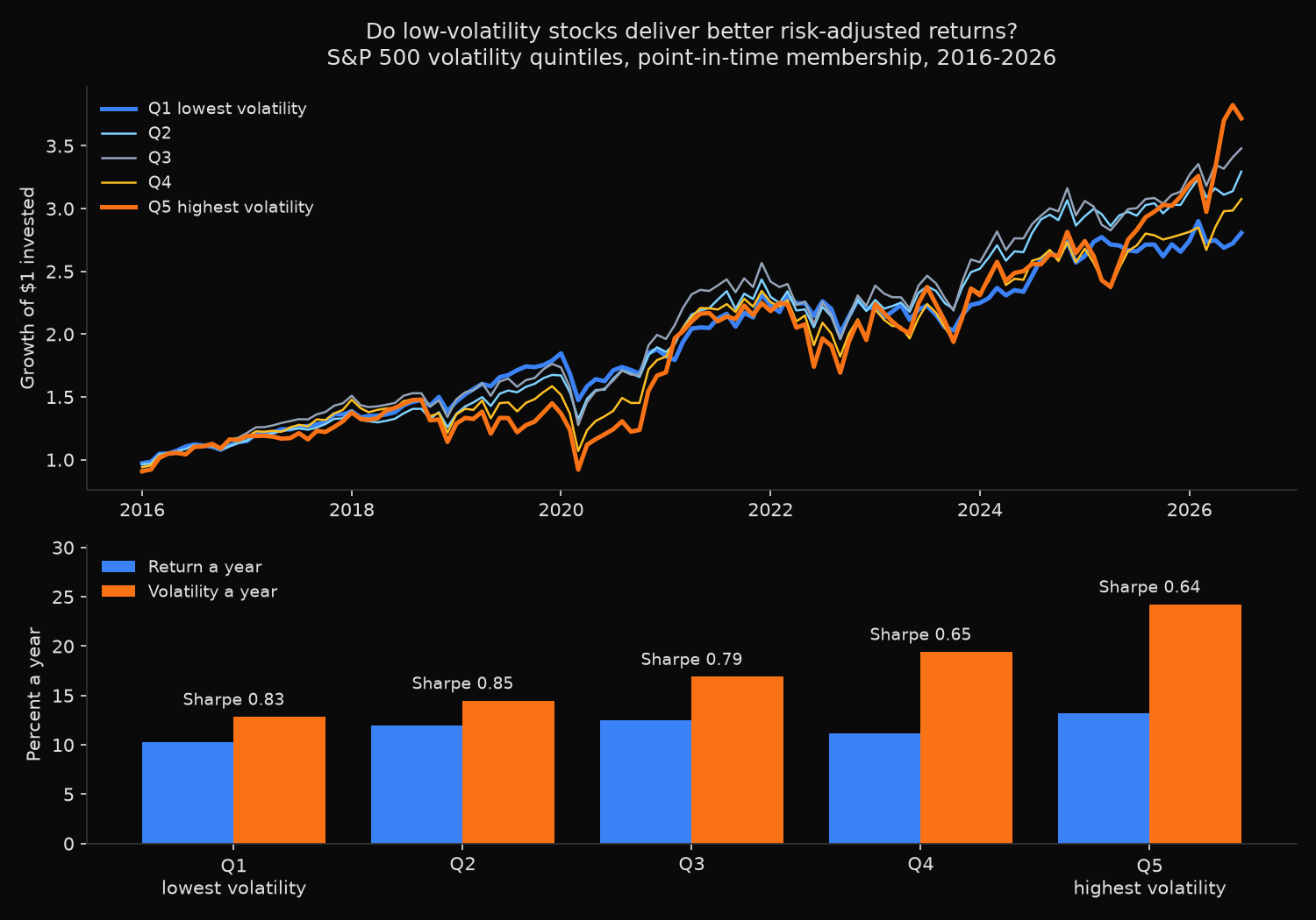
Point-in-time S&P 500 volatility quintiles, 2016-01 to 2026-07 (127 months)
Formation: annualised standard deviation of the trailing 36 monthly total returns, measured each 31 December
Portfolios: equal weighted, reformed every January, Sharpe taken without a risk-free deduction

11 membership snapshots cover 686 distinct companies; 5 set aside by the return-bound screen

Formation    Members  Ranked   Q1 vol   Q5 vol
2016             495     472    14.7%    34.1%
2017             496     481    15.3%    36.8%
2018             498     483    15.0%    36.1%
2019             499     485    15.5%    37.4%
2020             500     488    14.7%    36.9%
2021             500     484    19.6%    50.0%
2022             500     485    20.2%    50.7%
2023             499     486    22.8%    54.1%
2024             499     489    20.5%    45.1%
2025             499     487    19.8%    45.9%
2026             496     485    17.5%    44.6%

             Formation vol     CAGR  Ann vol  Sharpe  Worst mo   Max DD
Q1 lowest            17.8%   10.24%   12.83%    0.83    -12.5%   -20.2%
Q2                   22.1%   11.93%   14.47%    0.85    -14.1%   -21.2%
Q3                   25.7%   12.51%   16.90%    0.79    -19.1%   -27.7%
Q4                   30.7%   11.20%   19.42%    0.65    -21.8%   -32.6%
Q5 highest           42.9%   13.21%   24.23%    0.64    -25.6%   -37.7%
All ranked                   12.06%   16.64%    0.77    -18.6%   -27.2%

Calendar year total return (%)
            Q1      Q2      Q3      Q4      Q5     ALL
2016      14.0    13.4    17.5    15.8    15.6    15.3
2017      19.3    17.3    23.4    20.6    12.9    18.7
2018       1.8    -5.3    -7.6   -13.1   -12.6    -7.4
2019      29.2    33.1    31.6    30.6    27.0    30.6
2020       5.1    13.1    13.1    13.1    15.2    12.4
2021      23.5    28.5    28.7    30.7    34.6    29.5
2022      -5.2   -10.3   -13.3   -15.5   -13.1   -11.3
2023       1.4    14.2    16.6    19.7    20.9    14.6
2024      15.1    14.9    13.5     8.5    12.0    12.9
2025       3.3     5.7     6.4     8.5    17.1     8.4
2026       5.6     8.8    11.0    10.2    20.1    11.3

Q1 minus Q5: -6.38% a year, t = -0.83; Q1 ahead in 5 of 11 calendar years
  2016-2020  Q1 return 13.46% Sharpe  1.09   Q5 return 10.80% Sharpe  0.52
  2021-2026  Q1 return  7.44% Sharpe  0.61   Q5 return 15.42% Sharpe  0.75
Q1 geared 1.888x to Q5 volatility: 18.48% a year before financing cost, max drawdown -36.3%
Breakeven financing rate on the borrowed 0.888 of capital: 5.17% a year

2026 sector mix, lowest quintile: Utilities 22, Consumer Staples 17, Industrials 14, Financials 13
2026 sector mix, highest quintile: Information Technology 27, Consumer Discretionary 20, Health Care 13, Industrials 10
What this tells us
The sort works: the calmest fifth averaged 17.8% formation volatility and ran at 12.83% as a portfolio, the wildest 42.9% and 24.23%.
The strong claim fails. The wildest fifth compounded at 13.21% a year against the calmest fifth’s 10.24%, with the equal-weighted average of all ranked names between them at 12.06%, and the ordering across the middle quintiles is not clean. A monthly rebalanced position long the calmest fifth and short the wildest compounds at -6.38% a year, carrying a t-statistic of -0.83, so the disciplined reading is that raw returns are indistinguishable across the sort.
The weak claim holds, on every risk measure at once. Sharpe declines from 0.85 at Q2 to 0.64 at Q5, worst drawdown widens without interruption from 20.2% to 37.7%, and the worst month falls from -12.5% to -25.6%. Q1 gave up 2.97 points of annual return and removed 11.40 points of volatility for it.
Splitting the decade in half explains why practitioners argue about this. From 2016 to 2020, Q1 beat Q5 on return, 13.46% against 10.80%, and doubled its Sharpe, 1.09 against 0.52; textbook anomaly. From 2021 the ordering flipped, Q5 returning 15.42% at a Sharpe of 0.75 against Q1’s 7.44% at 0.61. Most of the reversal sits in 2025 and the first seven months of 2026, when the highest-volatility fifth (27 technology names, 20 consumer discretionary) rode the artificial intelligence trade and the calmest fifth (22 utilities, 17 staples) sat it out. Defence paid in 2018 and 2022, +1.8% against -12.6% and -5.2% against -13.1%.
So what?
Nobody should buy low volatility expecting a higher return. The evidence is absent here, and the five-year reversal shows what that belief costs when the market rewards risk for a stretch.
Buy it for the loss profile instead. Halving the worst month from -25.6% to -12.5% and cutting 17.5 points off the worst drawdown is what the quintile delivers, which matters most under a drawdown limit.
Where borrowing is permitted the comparison changes. Gearing Q1 by 1.888 times brings it to Q5’s volatility and to 18.48% a year before financing cost, 5.27 points ahead, at a shallower worst drawdown of 36.3%. The borrowed 0.888 of capital has to cost under 5.17% a year for that to hold, so the trade turns on the funding rate.
Rebuild the ranking every year on membership as it stood, and check sub-periods first: a full-sample average conceals a factor that ran at a Sharpe of 1.09 for five years and 0.61 for the next five.
Built with xfinlink — free financial data API for Python. pip install -U xfinlink
pip install -U xfinlink