
Has the Stock-Bond Correlation Flipped? 60/40 Portfolio Risk in Python
August 1, 2026
What's the question?
A 60/40 portfolio does not work because bonds are safe. It works because bonds have tended to move the other way when equities fall, and that opposition turns two risky holdings into one steadier book. Correlation measures that opposition: a number between -1 and +1 describing how closely two return series move together. At -0.4, a bad day for stocks is more often than not a decent day for Treasuries, so the bond leg absorbs part of the loss. At +0.1 it absorbs almost nothing.
Most risk models treat that number as a fixed property of the pair, estimated once from a long history and reused. If the sign has changed, a balanced portfolio carries more risk than its stated allocation implies, without anyone touching the weights.
Three questions follow: has the equity-Treasury correlation changed sign, when, and what does the change cost a 60/40 book?
The approach
Four exchange-traded funds stand in for the asset classes: SPY for US large cap equity, TLT for Treasuries of twenty years and longer, IEF for the seven to ten year part of the curve, and LQD for investment grade credit. The window runs from 29 July 2002, the first trading day the bond funds share, to 31 July 2026: 6,041 daily observations on a calendar common to all four.
- Pull daily total returns and keep only dates where every fund has an observation, so no correlation is computed across a misaligned calendar.
- Estimate the break date rather than assume it. Every interior day is tested as a candidate split, trimming 15% from each end, and the winner maximises the gap between the two sub-sample correlations after Fisher’s z transform, which makes that gap comparable across candidates.
- Measure correlation and annualised volatility in each sub-period, then rebuild the risk of a 60/40 book from the two-asset variance formula. Repeating that with the post-break volatilities and the old correlation isolates the correlation channel from the volatility channel.
- Test whether the correlation depends on the inflation environment, using the trailing one-year return of TIP minus IEF as a proxy for breakeven inflation.
Code
import numpy as np
import pandas as pd
import xfinlink as xfl

xfl.set_api_key("YOUR_API_KEY")  # free at https://xfinlink.com/signup

TICKERS = ["SPY", "TLT", "IEF", "LQD", "TIP"]
px = pd.concat([xfl.prices(t, start="2002-07-26", fields=["close", "return_daily"])
                for t in TICKERS])
wide = px.pivot_table(index="date", columns="ticker", values="return_daily")
d = wide[["SPY", "TLT", "IEF", "LQD"]].dropna()      # common calendar

def fisher(r):
    return 0.5 * np.log((1 + r) / (1 - r))

x, y, n = d["SPY"].values, d["TLT"].values, len(d)
scores = []
for i in range(int(n * 0.15), int(n * 0.85)):
    r1 = np.corrcoef(x[:i], y[:i])[0, 1]
    r2 = np.corrcoef(x[i:], y[i:])[0, 1]
    z = (fisher(r1) - fisher(r2)) / np.sqrt(1 / (i - 3) + 1 / (n - i - 3))
    scores.append((i, abs(z)))

split = max(scores, key=lambda s: s[1])[0]
BREAK = d.index[split]
pre, post = d[d.index < BREAK], d[d.index >= BREAK]

def port_vol(se, sb, rho, we=0.60):
    wb = 1 - we
    return np.sqrt(we**2 * se**2 + wb**2 * sb**2 + 2 * we * wb * rho * se * sb)

ann = np.sqrt(252)
se, sb = post["SPY"].std() * ann, post["TLT"].std() * ann
rho_pre, rho_post = pre["SPY"].corr(pre["TLT"]), post["SPY"].corr(post["TLT"])
print(BREAK.date(), round(rho_pre, 3), round(rho_post, 3))
print(round(port_vol(se, sb, rho_post) * 100, 2), round(port_vol(se, sb, rho_pre) * 100, 2))
Full script with formatting and visualisation: stock-bond-correlation-60-40-portfolio-risk-python.py
Output
Sample: 2002-07-29 to 2026-07-31  (6041 trading days)
Estimated break in the SPY/TLT correlation: 2020-08-04   |z| = 17.1
Split points within 1.0 of the peak: 2020-04-28 to 2022-08-02
Pre-break 4536 days, post-break 1505 days

                                  correlation with SPY
                                       pre      post    change
Long Treasuries (TLT)               -0.419    +0.063    +0.481
7-10y Treasuries (IEF)              -0.414    +0.077    +0.491
Investment grade credit (LQD)       +0.111    +0.365    +0.254

Share of 126-day windows with a positive SPY/TLT correlation:
  pre-break  10.2%
  post-break 54.2%

                                 annualised volatility
                                       pre      post
SPY                                 19.45%    16.82%
TLT                                 13.92%    15.29%
IEF                                  6.63%     7.30%

60/40 SPY/TLT, annualised volatility
  pre-break  : 10.62%   (realised 10.62%)
  post-break : 12.12%   (realised 12.12%)
  post-break volatilities at the old correlation of -0.419:  9.36%
  risk added by the correlation change alone: +2.77 pp
  diversification saving vs a weighted average of the two legs:  pre 6.62 pp,  post 4.09 pp

60/40 SPY/IEF, annualised volatility
  pre-break  : 10.84%   (realised 10.84%)
  post-break : 10.72%   (realised 10.72%)
  post-break volatilities at the old correlation of -0.414:  9.27%
  risk added by the correlation change alone: +1.45 pp
  diversification saving vs a weighted average of the two legs:  pre 3.48 pp,  post 2.29 pp

SPY/TLT correlation by trailing 1-year breakeven inflation proxy (TIP minus IEF)
  bucket           n     corr   share after break
  Q1 lowest     1362   -0.415                 1%
  Q2            1361   -0.371                18%
  Q3            1361   -0.190                36%
  Q4 highest    1362   -0.128                56%
  same buckets, pre-break sample only (3941 days):
  Q1 lowest      986   -0.419
  Q2             985   -0.389
  Q3             985   -0.473
  Q4 highest     985   -0.459
What this tells us
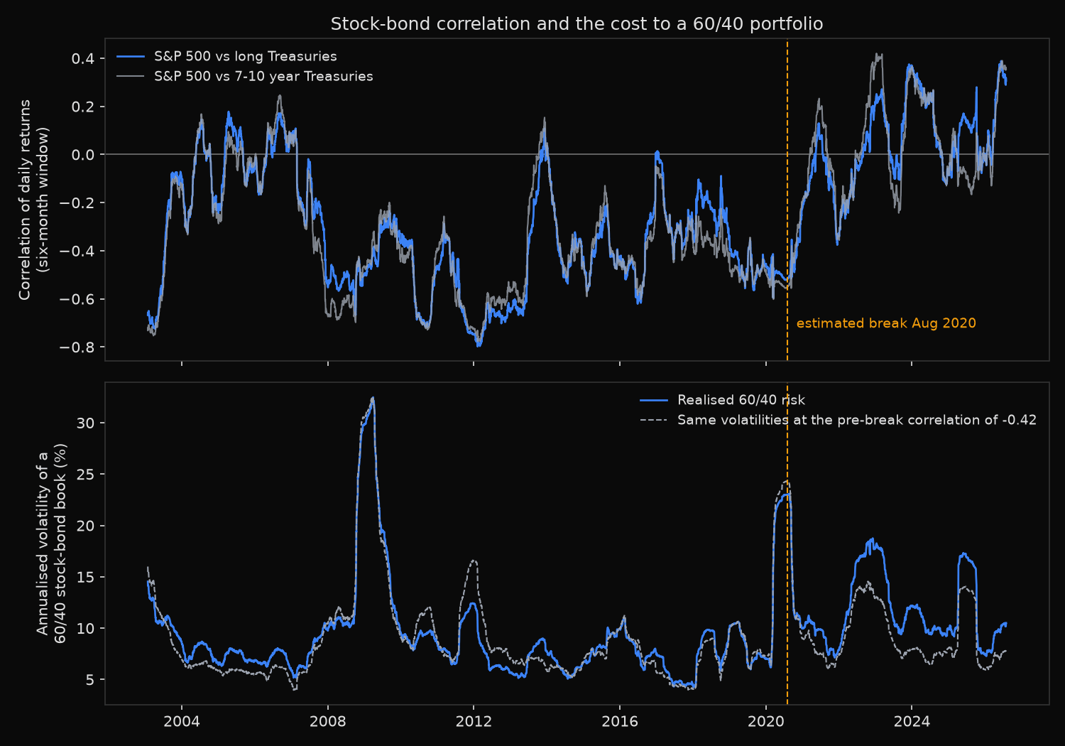
The sign has flipped. Equity and long Treasury returns correlated at -0.419 across the 4,536 trading days before the estimated break and at +0.063 across the 1,505 days after it, and the shorter part of the curve moved almost identically, from -0.414 to +0.077. A z-statistic of 17.1 rules out sampling noise.
The date is less precise than the sign. Every split point between April 2020 and August 2022 scores within one unit of the peak, so the transition spans roughly two years rather than a single day. Before the break, 10.2% of six-month windows showed a positive correlation; after it, 54.2%.
The SPY/IEF pair shows why headline volatility is a poor alarm. That book ran at 10.84% before the break and 10.72% after, apparently unchanged. Rebuilt with the post-break volatilities and the old correlation it would have run at 9.27%, so equity volatility falling from 19.45% to 16.82% concealed 1.45 points of lost diversification. The long-duration version hid nothing, moving from 10.62% to 12.12%, and that figure is reproducible from the table: 0.36 times 16.82 squared plus 0.16 times 15.29 squared plus 0.48 times 0.063 times 16.82 times 15.29 gives 147, whose square root is 12.1. Replace 0.063 with -0.419 and the same volatilities produce 9.36%.
Inflation looks like the explanation until the sample is split. Correlations sorted by the trailing breakeven proxy run from -0.415 in the lowest bucket to -0.128 in the highest, but 56% of the highest bucket falls after the break against 1% of the lowest. Inside the pre-break sample the ordering disappears: -0.419, -0.389, -0.473 and -0.459. The full-sample pattern reflects the regime change, not the inflation environment.
So what?
Any risk model still carrying a stock-bond correlation near -0.4 understates the risk of a balanced book by roughly a quarter when the bond leg is long duration. Re-estimate on a rolling two-year window and use the measured number.
Rebalancing toward credit makes the problem worse, since LQD moved from +0.111 against equities to +0.365. The uncomfortable result sits in the volatility column: post-break, no mix of SPY and TLT reaches the 10.62% the old 60/40 delivered. The minimum-variance blend of those two funds holds 44.9% equity and still runs 11.66%, because long Treasuries themselves grew more volatile, from 13.92% to 15.29%. Getting back to the old risk level takes a genuinely low-volatility asset in place of duration, which in practice means cash or bills; 63% equity against a zero-volatility remainder returns the book to 10.62%.
Run the break search on whichever pairs carry the portfolio’s diversification, and check that the hedge being paid for still works.
Built with xfinlink — free financial data API for Python. pip install -U xfinlink
pip install -U xfinlink